Week 3, lecture 7

Learning objectives

After following this lecture, you will be able to:

Identify the conditions that lead to bound and scattering states for a given potential.
Apply the relevant boundary conditions to specify the allowed wavefunctions and energies.
Represent graphically the wavefunctions in potentials that combine scattering and bound states.

Bound and scattering states¶

Up to now, we have been seen two different kinds of quantum systems:

The first kind of system are those which involve confining potentials, such as the infinite square well and the harmonic oscillator. These systems are characterised by the fact that the wave function $\psi(x)$ vanishes for all allowed quantum states in the $|x|\rightarrow \infty$ limit.

The quantum states for systems involving confining potentials have associated both quantized wavefunctions and energies. In other words, for such systems all the allowed quantum states are bound states.

Note

A confining potential, such as the harmonic oscillator or the infinite barrier, satisfies that $V(x)\to \infty$ for $x\to \pm \infty$. This implies that for large enough values of $|x|$ one will have that $E < V(x)$, no matter the value of $E$. As we will see later, this configuration corresponds to a classically forbidden region where the wave function is exponentially suppressed.

The second kind of system that we have discussed is the free particle, where on the contrary none of the wave functions nor the energies were quantised, but rather we found a continuous spectrum of states and energies.

For a free particle of well-defined energy, the wave function $\psi(x)\neq 0$ is finite when taking the limit $|x|\rightarrow \infty$. We denote quantum states that do not vanish at infinity as scattering states.

Therefore, so far we have discussed quantum systems where either all states were quantised (that is, the complete spectrum was composed by bound states) or none of them were (that is, the complete spectrum was composed by scattering states).

In this lecture, we will discuss quantum systems characterised by potentials that lead to the presence of both scattering and bound states, depending on the value of the particle energy $E$.

The delta function potential¶

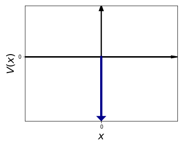
In the following, we are going to illustrate this class of quantum systems by considering the delta function potential $V(x)$, defined by

\[V(x)=-\alpha \delta (x)\]

where $\alpha$ is a positive real constant.

Info

Recall that $\delta(x)$ is the Dirac delta function, that despite its name it is a distribution rather than a function, and which is defined by its action within an integral $$ \int_{-\infty}^{\infty} dx~\delta(x-a)f(x) = f(a)$$ for any value of the constant $a$.

While such potential does not correspond to any physical quantum system, it makes possible highlighting the main features of quantum states that exhibit both bound and scattering states. As we will show below, this potential leads to a single bound state for $E<0$ and then to an infinite number of scattering states for positive energies, $E>0$.

Below we show the Dirac delta function potential $V(x)=-\alpha \delta(x)$.

This delta function potential can be understood as the limit of an infinitely narrow and deep finite square potential barrier whose area is kept constant. That is, if we have a potential such that $$ V(x) = - |V_0| \quad {\rm for } \quad -L \le x \le L $$ $$ V(x) = 0 \quad {\rm for } \quad |x|> L $$ then the Dirac delta function is obtained if one takes the limit $|V_0|\to \infty$ and $L \to 0$ while keeping the product $\alpha = 2|V_0|L$ fixed.

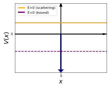
As displayed below, for this kind of potentials (both for the Dirac delta and for the Coulomb case) we will have two possible situations depended on the value of the energy $E$ of the particle moving in this potential:

For $E>0$, we have that $\forall x$ that $E > V(x)$. This implies a configuration that is similar to the free particle, and the solutions of the Schroedinger equation for $E>0$ correspond to scattering states that do not vanish at infinity.
For $E<0$, one sees instead that for large enough values of $|x|$ one ends up with $E<V(x)$, which is the classically forbidden region (indicated by the dashed purple line). The solutions to the Schroedinger equation for $E<0$ in this case correspond to bound states that decay exponentially fast in the $|x|\to \infty$ limit.

We also see how for $E<0$ there is a very narrow classically allowed region where $E>V(x)$ (solid purple line), and there the wave function will display an oscillatory behaviour instead.

In the following, we quantify these statemenets by solving explicitely the Schroedinger equation for $E>0$ (scattering states) and for $E<0$ (bound states).

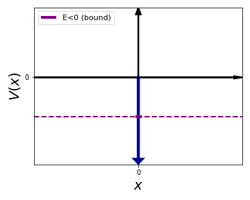
Bound states¶

Let's start by considering bound states with $E<0$. As we will show, the case of the delta function potential is special since there will be a single bound state. For other potentials, such as the Coulomb potential, in general there will be a large (maybe even infinite) number of allowed bound states. We are considering the configuration shown schematically below:

For both $x<0$ and $x>0$ we can easily solve the Schroedinger equation, since it is nothing but the free particle equation. Indeed, in these regions we have a vanishing potential, recall that the Delta function potential $V(x) = -\alpha \delta(x)$ vanishes everywhere except for $x=0$. Since the energy is negative, we will make this explicit by taking the absolute value and writing the Schroedinger equation as:

\[-\frac{\hbar^2}{2m}\frac{d^2\psi(x)}{dx^2}=-|E|\psi(x)\]

and then using the free-particle solutions we can write

For $x>0$: $\quad \psi_+(x)=Ae^{\sqrt{\frac{2m|E|}{\hbar^2}}x}+Be^{-\sqrt{\frac{2m|E|}{\hbar^2}}x}=Ae^{kx}+Be^{-kx}$

For $x<0$: $\quad \psi_-(x)=Ce^{\sqrt{\frac{2m|E|}{\hbar^2}}x}+De^{-\sqrt{\frac{2m|E|}{\hbar^2}}x}=Ce^{kx}+De^{-kx}$

where as usual we have defined $k\equiv \sqrt{2m|E|/\hbar^2}$.

The consequence of the negative energy of the particle is that now we do not have the oscillatory behaviour typical of the free particle but rather we have real exponentials. Note also that we have to be careful to separate the $x>0$ and $x<0$ regions, since these are separated by the delta function potential that arises at $x=0$.

Info

The wavefunction $\psi(x)$ is always continuous everywhere in $x$, but its first derivative $d\psi(x)/dx$ is only continuous in regions of $x$ where the potential function $V(x)$ is finite. Both properties follow directly from the structure of the Schroedinger equation.

In order to determine the integration constants $A$, $B$, $C$, and $D$ we need to impose the boundary conditions for the wave function:

The wavefunction must be normalizable because it corresponds to a bound state, and therefore the following condition needs to be satisfied: $\psi(x)\rightarrow 0$ when $x\rightarrow \pm \infty$. Imposing this condition leads to:

For $x>0$: $\psi_+(x)=Be^{-\sqrt{\frac{2m|E|}{\hbar^2}}x}$, since $A=0$ because $e^x$ blows up at $x \to +\infty$.

For $x<0$: $\psi_-(x)=Ce^{\sqrt{\frac{2m|E|}{\hbar^2}}x}$, since $D=0$ because $e^{-x}$ blows up at $x \to -\infty$.
The wavefunction (solution of the Schroedinger equation) is always continuous everywhere in space. This requirement leads to $\psi_+(x=0)=\psi_-(x=0)$ and imposing this condition we have that $B=C$.

Taking into account these two relations, we have that for the delta function potential the wave function of the bound states will be given by

\[\psi_+(x)=Be^{-\sqrt{\frac{2m|E|}{\hbar^2}}x} \, , \quad x >0\]

\[\psi_-(x)=Be^{\sqrt{\frac{2m|E|}{\hbar^2}}x} \, , \quad x<0\]

with $B$ some normalisation constant.

As mentioned above, in general the first derivative of the wave function is only continous for potentials that are finite everywhere in space. In regions of $x$ where the potential $V(x)$ that are locally infinite the first derivative of the wave function will be discontinous. So for quantum systems such as the Dirac delta potential we cannot use the continuity of the first derivative of $\psi(x)$ to fix the normalisation constant $B$.

Info

It can be shown from the Schroedinger equations that the first derivative of the wavefunction satisfies:

\[\frac{d\psi(x)}{dx}\Big|_{x_0-\epsilon}^{x_0+\epsilon}=\frac{2m}{\hbar^2}\int_{x_0-\epsilon}^{x_0+\epsilon}V(x)\psi(x)dx\]

for any potential $V(x)$. This property means that the derivative of the the wave function $\psi(x)$ is only continuous for finite potentials. To derive this relation, note that the Schroedinger equation can always be expressed as

\[\frac{d^2\psi(x)}{dx^2} = \frac{2m}{\hbar^2}\left( V(x)-E\right)\psi(x)\]

and now if you integrate between $x_0-\epsilon$ and $x_0+\epsilon$ and take the limit $\epsilon\to 0$ you obtain the relation above, since the second derivative integrates to the first derivative and the term proportional to $E$ goes to zero in this limit (since $\psi(x)$ is a continous function everywhere ).

In the case of the delta function potential, the derivative of $\psi(x)$ will not be continuous, but we can nevertheless evaluate the discontinuity and use the property above to fix the boundary condition $B$. Evaluating the discontinuity of the wave function at $x_0=0$ leads to

\[\frac{d\psi(x)}{dx}\Big|_{-\epsilon}^{\epsilon}=\frac{2m}{\hbar^2}\int_{-\epsilon}^{+\epsilon}V(x)\psi(x)dx=-\alpha\frac{2m}{\hbar^2}\int_{-\epsilon}^{+\epsilon}\delta(x)\psi(x)dx=\]

\[=-\frac{2m\alpha}{\hbar^2}\psi(0)=-\frac{2m\alpha}{\hbar^2}B\]

Now that we know the value of the discontinuity at $x=0$, we can impose this boundary condition to fix the value of the integration constant $B$

\[\frac{d\psi_+(x)}{dx}=-B\sqrt{\frac{2m|E|}{\hbar^2}}e^{-\sqrt{\frac{2m|E|}{\hbar^2}}x} \,\to \,\frac{d\psi_+(0)}{dx}=-B\sqrt{\frac{2m|E|}{\hbar^2}}\]

\[\frac{d\psi_-(x)}{dx}=B\sqrt{\frac{2m|E|}{\hbar^2}}e^{\sqrt{\frac{2m|E|}{\hbar^2}}x} \, \to \, \frac{d\psi_-(0)}{dx}=B\sqrt{\frac{2m|E|}{\hbar^2}}\]

\[\frac{d\psi_+(0)}{dx}-\frac{d\psi_-(0)}{dx}=-2B\sqrt{\frac{2m|E|}{\hbar^2}}\]

Putting together this information one obtains the following relation:

\[-2B\sqrt{\frac{2m|E|}{\hbar^2}}=-\frac{2m\alpha}{\hbar^2}B\]

\[\sqrt{\frac{2m|E|}{\hbar^2}}=\frac{m\alpha}{\hbar^2}\]

\[|E|=\frac{m\alpha^2}{2\hbar^2}\]

Therefore, we have demonstrated that in the case of the Dirac delta function potential there is a single bound state with energy $E=-m\alpha^2/2\hbar^2$. This is the only value of the energy for which all the boundary conditions of the problem are satisfied.

Note that in general we will have more than a bound state in this kind of systems, the delta function potential is special in this respect.

Exercise: determine explicitely the value of the integration constant $B$ of the bound state wave function by imposing that the wave function is normalised. You should find this normalisation constant is given by $B=(\sqrt{2m|E|}/\hbar)^{1/2}$.

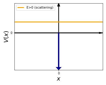
Scattering states¶

Following this discussion of the single bound state of the Dirac delta potential, we now consider the case of scattering states with positive energy $E>0$, a configuration which is depicted below:

As in the case of the bound states, we now need to solve the Schroedinger equation separately for the $x<0$ and for the $x>0$ regions:

\[-\frac{\hbar^2}{2m}\frac{d^2\psi(x)}{dx^2}=|E|\psi(x)\]

where we have made explicit the fact that the energy is now positive (note the absolute value).

The solutions to this equation are of the same form as those of the free particle:

For $x>0$: $\quad \psi_+(x)=Ae^{i\sqrt{\frac{2m|E|}{\hbar^2}}x}+Be^{-i\sqrt{\frac{2m|E|}{\hbar^2}}x}=Ae^{ikx}+Be^{-ikx}$

For $x<0$: $\quad \psi_-(x)=Ce^{i\sqrt{\frac{2m|E|}{\hbar^2}}x}+De^{-i\sqrt{\frac{2m|E|}{\hbar^2}}x}=Ce^{ikx}+De^{-ikx}$

where $k\equiv \sqrt{2m|E|}/\hbar$, namely an oscillatory behaviour that implies that the wave function remains non-zero for $|x|\to \infty$, as characteristic of scattering states.

Recall

Scattering states are not normalisable, and therefore we should not use the normalisation condition to fix any of the integration constants $A$, $B$, $C$, or $D$ or to determine the behaviour of the wave function in the $|x|\to \infty$ limit.

We now need to impose the boundary conditions on the wave function in order to determine the integration constants:

The wave function is always continuous:

\[\psi_+(x=0)=\psi_-(x=0)\]

\[A+B=C+D;~~{\rm Eq.}~[1]\]

The first derivative of the wave function will be discontinous but we can evaluate the expected value of the discontinuity. Using the same strategy as for the case of the bound state, the relation that needs to be imposed is:

\[\frac{d\psi_+(0)}{dx}-\frac{d\psi_-(0)}{dx}=-\frac{2m\alpha}{\hbar^2}\psi(0)=-\frac{2m\alpha}{\hbar^2}(A+B)\]

where

\[\frac{d\psi_+(0)}{dx}=ikA-ikB \, \quad \frac{d\psi_-(0)}{dx}=ikC-ikD\]

and therefore we end up with the following constraint:

\[ik(A-B-C+D)=-\frac{2m\alpha}{\hbar^2}(A+B);~~{\rm Eq.}~[2]\]

Eq. [1] and Eq. [2] are the two conditions that need to be satisfied by the coefficients of the wavefunctions correspinding to the scattering states of the Dirac delta function potential.

Warning

In this problem we have solved the Schroedinger equation for the delta potential assuming incident plane waves with fixed values of the energy. While these plane waves are not normalisable, they allow us to extract physically relevant information about the system such as the transmission and reflection coefficients, which only depend on the ratio of the intensities of the transmitted and reflected waves over the incident one, respectively. A full calculation of the solution would involve using physical wave packets but would not change the main results and thus it is not necessary at this point.

We can represent graphically below the physical interpretation of the four components of the scattering wave function. The terms $Ce^{ikx}$ and $Ae^{ikx}$ correspond to particles propagating from left to right, while the terms $De^{-ikx}$ and $Be^{-ikx}$ correspond instead to particles propagating from right to left. The effect of the potential is seen by the fact that in general $C\ne A$ and $D \ne B$.

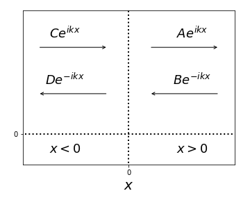
In a realistic situation, we would have a particle approaching the potential from a single direction, let us say from the left. We then call the component $Ce^{ikx}$ as the incident wave. The particle then interacts with the potential and results into a transmitted wave ($Ae^{ikx}$) and a reflected wave ($De^{-ikx}$). Therefore, for this specific scenario we have to impose that $B=0$.

Now we realise that we have two equations (Eq. [1] and Eq. [2]) coming from the boundary conditions and three unknowns ($A$, $C$, and $D$), so we can solve the equations in terms of a single parameter. We can express the coefficients $A$ (of the transmitted wave) and $D$ (of the reflected wave) in terms of $C$ (the incident wave):

\[D=\frac{i\frac{m\alpha}{k\hbar^2}}{1-\frac{im\alpha}{k\hbar^2}}C\]

\[A=\frac{1}{1-\frac{im\alpha}{k\hbar^2}}C\]

It is convenient to define transmission $T$ and reflection $R$ coefficients as follows:

\[T\equiv\frac{|A|^2}{|C|^2};~~{\rm Eq.~}[3]\]

\[R\equiv\frac{|D|^2}{|C|^2};~~{\rm Eq.~}[4]\]

since recall that in quantum theory probabilities are constructed from the square of the wave function, rather than from the wave function itself. In other words, $T$ indicates the probability that the particle is transmitted through the potential while $R$ indicates the probability that it is reflected.

In our particular case, the transmission and refection coefficitents turn out to be:

\[T=\frac{1}{1+\beta^2}\]

\[R=\frac{\beta^2}{1+\beta^2}\]

where we have defined $\beta\equiv\frac{m\alpha}{k\hbar^2}$

Example

For a very energetic particle, $k\rightarrow\infty$, then we have that $\beta\rightarrow 0$, and therefore $T\rightarrow 1$ and $R\rightarrow 0$: the particle is almost certain to be transmitted through the potential, which makes sense intuitively. Likewise, if $\alpha \to \infty$ then $\beta \to \infty$ and hence $T\to 0$ and $R\to 1$: the particle will bounce and will be fully reflected by the potential, with a vanishing probability of transmission.

Exercise: evaluate explicitely the sum $R+T$ and justify the obtained result.