The Harmonic Oscillator

Week 2, Lectures 5 & 6

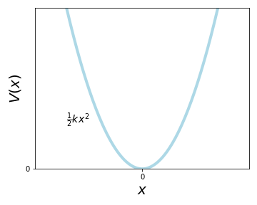
We will now focus on a different potential: the harmonic oscillator (HO). This is of course a very well known system from classical mechanics and its potential is described by a parabola \(V=\frac{1}{2}kx^2\). Physically it can be represented by a mass on a spring with the restoring force \(F=-kx\).

Note

The harmonic oscialltor is a very useful pronlem to study in physics, as almost anything that has a small deviation from its equilibrium behaves like a harmonic oscillator. Take for example this admittedly weird potential: GRAPH

In general this is very hard to solve of course. However, for a particle in a (local) potential minimum and for small displacements this behaves like a HO. We can do a Taylor expansion

\[V(x)=V_0+\frac{\mathrm{d}V}{\mathrm{d}x}(x-x_0)+\frac{1}{2}\frac{\mathrm{d}^2V}{\mathrm{d}x^2}(x-x_0)^2+\dots\]

The linear term is zero because we have assumed we are in a minimum, while the quadratic term is very similar to the HO potential!

So how does the HO work in QM? Let us take the TISE and use \(V=\frac{1}{2}kx^2=\frac{1}{2}m\omega^2x^2\), with \(\omega=\sqrt{\frac{k}{m}}\)

\[-\frac{\hbar^2}{2m}\frac{\mathrm{d}^2\psi}{\mathrm{d}x^2}+\frac{1}{2}m\omega^2x^2\psi=E\psi\]

There are two alternative approaches on how to solve the SE: through an algebraic approach (essentially clever guessing and then deriving the solution, see Book) or an operator approach, which is a what we will follow here. This is also a good way to start working with operators in general and see how they differ from normal variables.

Recap

Take for example the momentum \(p\), which is a simple number in classical physics. In QM however, it's described by an operator \(\hat{p}=\frac{\hbar}{i}\frac{\mathrm{d}}{\mathrm{d}x}\). In order to get to a value for the momentum, we have to calculate the expectation value \(\langle p\rangle=\int\psi^*\hat{p}\psi\mathrm{d}x\). We put "hats" on the operators to clearly distinguish them from numbers.

Let's start by writing down the Hamiltonian for the harmonic oscillator

\[\hat{H}=\frac{\hat{p}^2}{2m}+\frac{1}{2}m\omega^2\hat{x}^2=\frac{1}{2m}\left(\hat{p}^2+(m\omega\hat{x})^2\right)\]

We can try to rewrite this as a sum of squares using complex numbers \(u^2+v^2=(u+iv)(u-iv)=u^2+ivu-iuv+v^2\), where \(ivu-iuv\) is zero if \(u,v\) are just numbers. We can now substitute these numbers with operators \(v=\hat{p}\) and \(u=m\omega\hat{x}\)

\[\left(i\hat{p}+m\omega\hat{x}\right)\left(-i\hat{p}+m\omega\hat{x}\right)=\hat{p}^2+i\hat{p}m\omega\hat{x}-im\omega\hat{x}\hat{p}+(m\omega\hat{x})^2=\]

\[=2m\left\{\frac{\hat{p}^2}{2m}+\frac{1}{2}m\omega^2\hat{x}^2\right\}+im\omega\left[\hat{p}\hat{x}-\hat{x}\hat{p}\right]\]

The term in the curly brackets is the Hamiltonian \(\hat{H}\), while the extra term in the square brackets should be zero - if \(\hat{x}\) and \(\hat{p}\) were numbers. But as they are operators, we have to verify this by applying them to a test function (which we'll choose to call \(\psi\))!

\[\hat{x}\hat{p}\psi=x\frac{\hbar}{i}\frac{\mathrm{d}}{\mathrm{d}x}\psi\]

\[\hat{p}\hat{x}\psi=\frac{\hbar}{i}\frac{\mathrm{d}}{\mathrm{d}x}x\psi=\frac{\hbar}{i}\left(\psi+x\frac{\mathrm{d}}{\mathrm{d}x}\psi\right)\]

\[\left(\hat{p}\hat{x}-\hat{x}\hat{p}\right)\psi=\frac{\hbar}{i}\left(\psi+x\frac{\mathrm{d}}{\mathrm{d}x}\psi-x\frac{\mathrm{d}}{\mathrm{d}x}\right)=\frac{\hbar}{i}\psi\]

Interestingly, the extra term is not zero but \(\hat{p}\hat{x}-\hat{x}\hat{p}=-i\hbar\)! It is called the commutator of \(\hat{x}\) and \(\hat{p}\), a concept that is very different to classical physics. The commutator of two operators \(\hat{A}\) and \(\hat{B}\) is usually written as \(\left[\hat{A},\hat{B}\right]=\hat{A}\hat{B}-\hat{B}\hat{A}\). If \(\left[\hat{A},\hat{B}\right]=0\) we say that \(\hat{A}\) and \(\hat{B}\) commute. In quantum mechanics, it is very important to know if two operators commute! The position and momentum of a particle do not commute, as we have just seen \(\left[\hat{x},\hat{p}\right]=i\hbar\). Similarly to matrices, the order of operators matters!

Let us come back to our Hamiltonian and define

\[\hat{a}_+=\frac{1}{\sqrt{2\hbar m\omega}}\left(-i\hat{p}+m\omega\hat{x}\right)\]

\[\hat{a}_-=\frac{1}{\sqrt{2\hbar m\omega}}\left(+i\hat{p}+m\omega\hat{x}\right)\]

which allows us to rewrite \(\hat{H}=\hbar\omega\left(\hat{a}_+\hat{a}_-+\frac{1}{2}\right)\), as \(\hat{x}\) and \(\hat{p}\) don't commute. The commutator of \(\left[\hat{a}_-,\hat{a}_+\right]=1\) (check at home!). How does this help us to solve the TISE? In fact, \(\hat{a}_+\) and \(\hat{a}_-\) have some very interesting properties, that we will use to find the solutions of the HO potential.

Lemma

If we have a solution \(\psi\) of the SE with the harmonic oscillator potential with energy \(E\), then \(\hat{a}_+\psi=\psi'\), where \(\psi'\) is also a solution of the SE, with an energy \(E'=E+\hbar\omega\).

Let us now proof that \(\hat{H}\psi=E\psi\rightarrow\hat{H}\psi'=E'\psi'\)

\[\hat{H}\psi'=\hat{H}\hat{a}_+\psi=\hbar\omega\left(\hat{a}_+\hat{a}_-+\frac{1}{2}\right)\hat{a}_+\psi=\hbar\omega\left(\hat{a}_+\hat{a}_-\hat{a}_++\frac{\hat{a}_+}{2}\right)\psi=\]

\[=\hbar\omega\hat{a}_+\left(\hat{a}_-\hat{a}_++\frac{1}{2}\right)\psi=\hbar\omega\hat{a}_+\left(1+\hat{a}_+\hat{a}_-+\frac{1}{2}\right)\psi=\hbar\omega\hat{a}_+\left(\hat{H}/\hbar\omega+1\right)\psi=\]

\[=\hbar\omega\hat{a}_+\left(E/\hbar\omega+1\right)\psi=\hbar\omega\left(E/\hbar\omega+1\right)\hat{a}_+\psi=\left(E+\hbar\omega\right)\psi'\]

Here we have used the commutator of \(\hat{a}_+\) and \(\hat{a}_-\), from which follows that \(\hat{a}_-\hat{a}_+=1+\hat{a}_+\hat{a}_-\). Clearly, if we let \(\hat{a}_+\) onto a solution, we get another solution with different energy. We can similarly prove that \(\hat{a}_-\psi\) is a solution with \(E'=E-\hbar\omega\) (check at home)! Because of these properties, \(\hat{a}_+\) and \(\hat{a}_-\) are called raising and lowering operators, respectively, and ladder operators as a general term for both. It's very interesting to note that these solutions all have equal energy spacing \(\Delta E=\hbar\omega\).

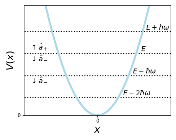
If we now have a single solution, we can get all solutions by simply applying the ladder operators! How can we find such a starting point? One important observation is that if we keep applying \(\hat{a}_-\) we can get to negative energies! And with negative energies you will actually not be able to get a normalizable wavefunction (see later). So the solution to this problem is that while \(\hat{a}_-\psi\) will always give a solution to the TISE, it will not necessarily be a physical one. And there is one trivial solution \(E=0\), which we usually reject, as it does not represent a particle. So we can simply define \(\psi_0\) as our last meaningful, physical solution, which we will call the ground state. This is the lowest energy state inside the well (the HO potential). Then \(\hat{a}_-\psi_0=0\)!

\[\hat{a}_-\psi_0=\frac{1}{\sqrt{2m\hbar\omega}}\left(i\frac{\hbar}{i}\frac{\mathrm{d}}{\mathrm{d}x}+m\omega x\right)\psi_0=0\]

We hence need to find a function of the form \(\frac{\mathrm{d}\psi_0}{\mathrm{d}x}=-\frac{m\omega x}{\hbar}\psi_0\), or simply \(\frac{\mathrm{d}f}{\mathrm{d}x}=-xf\). What about \(f=e^{-x^2/2}\)? We can hence write our wavefunction \(\psi_0\)

\[\psi_0(x)=A_0e^{-\frac{m\omega}{2\hbar}x^2}\]

The ground state is a Gaussian function with an energy \(E_0=\frac{1}{2}\hbar\omega\)! Now that we have the general form of \(\psi_0\), all we need to do is apply \(\hat{a}_+\) and we will get all other solutions

\[\psi_n(x)=A_n(\hat{a}_+)^n\psi_0(x)\]

\[E_n=\left(n+\frac{1}{2}\right)\hbar\omega\]

What about the normalization? We of course know \(\int_{-\infty}^{+\infty}|\psi_0(x)|^2\mathrm{d}x=1\) and \(\int_{-\infty}^{+\infty}e^{ax^2}\mathrm{d}x=\sqrt{\frac{\pi}{a}}\), hence \(A_0=\sqrt[4]{\frac{m\omega}{\pi\hbar}}\)

\[\psi_n(x)=\sqrt{\frac{1}{n!}}\left(\frac{m\omega}{\pi\hbar}\right)^{1/4}(\hat{a}_+)^ne^{-\frac{m\omega}{2\hbar}x^2}\]

Let us have a look at the solutions

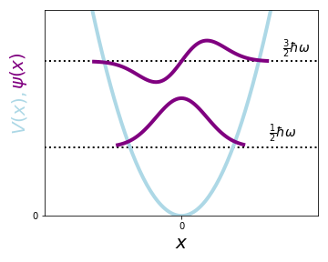
One thing that is interesting is that the potential barrier is not a hard barrier like it was for the infinite square well. This is also something that we wouldn't expect from classical physics: the particle should be confined to the well, however in QM it can be, with a very small probability, anywhere outside (exponentially smaller)! We also notice that the wavefunctions are in general Gaussian functions multiplied with Hermite polynomials.

Example:

Find \(\langle x\rangle=\int\psi_n^*\hat{x}\psi_n\mathrm{d}x\). We can do this the hard way, or we can use operators. For this it is convenient to define

\[\hat{x}=\sqrt{\frac{\hbar}{2m\omega}}\left(\hat{a}_++\hat{a}_-\right)\]

\[\hat{p}=i\sqrt{\frac{\hbar m\omega}{2}}\left(\hat{a}_+-\hat{a}_-\right)\]

This is very useful, as we know how \(\hat{a}_+\) and \(\hat{a}_-\) act on the \(\psi_n\)'s

\[\hat{a}_+\psi_n=\sqrt{n+1}\psi_{n+1}\]

\[\hat{a}_-\psi_n=\sqrt{n}\psi_{n-1}\]

Example:

Calculate \(\langle x\rangle\) for \(\psi_0(x)\).

\[\langle x\rangle=\int\psi_0^*\hat{x}\psi_0\mathrm{d}x=\sqrt{\frac{\hbar}{2m\omega}}\int\psi_0^*\left(\hat{a}_++\hat{a}_-\right)\psi_0\mathrm{d}x=\]

\[=\sqrt{\frac{\hbar}{2m\omega}}\int\psi_0^*\left(\sqrt{1}\psi_1+0\right)\mathrm{d}x=\sqrt{\frac{\hbar}{2m\omega}}\int\psi_0^*\psi_1\mathrm{d}x=0\]

Here we have used the orthogonality of the solutions. This result is of course expected, as the wavefunction is symmetric around zero.

Example:

Find \(\langle x\rangle\) for \(\psi=\frac{1}{\sqrt{2}}\left(\psi_0+\psi_1\right)\).

\[\langle x\rangle=\int\psi^*\hat{x}\psi\mathrm{d}x=\sqrt{\frac{\hbar}{8m\omega}}[\int\psi_0^*\left(\hat{a}_++\hat{a}_-\right)\psi_0\mathrm{d}x+\int\psi_0^*\left(\hat{a}_++\hat{a}_-\right)\psi_1\mathrm{d}x+\]

\[+\int\psi_1^*\left(\hat{a}_++\hat{a}_-\right)\psi_0\mathrm{d}x+\int\psi_1^*\left(\hat{a}_++\hat{a}_-\right)\psi_1\mathrm{d}x]=\]

If we look closely, due to the orthogonality of the solutions of the TISE, only one term in the second and third integral are non-zero.

\[=\sqrt{\frac{\hbar}{8m\omega}}(1+1)=\sqrt{\frac{\hbar}{2m\omega}}\]

Example:

Let us go back to the time dependent solutions and look at an example we have already calculated at the end of week 1: a particle is prepared in a superposition state: \(\Psi(x,0)=c_1\psi_1+c_2\psi_2\). The \(\psi_n\)'s and \(c_n\)'s can be chosen to be real if they are in a bound state, like they are in the HO potential. Obtaining \(\Psi(x,t)\) is easy: \(\Psi(x,t)=c_1e^{-iE_1t/\hbar}\psi_1+c_2e^{-iE_2t/\hbar}\psi_2\). And for \(|\Psi(x,t)|^2\) we need to calculate:

\[|\Psi(x,t)|^2=\left(c_1e^{iE_1t/\hbar}\psi_1+c_2e^{iE_2t/\hbar}\psi_2\right)\left(c_1e^{-iE_1t/\hbar}\psi_1+c_2e^{-iE_2t/\hbar}\psi_2\right)=\]

\[=c_1^2\psi_1^2+c_2^2\psi_2^2+c_1c_2\left(e^{-i(E_2-E_1)t/\hbar}+e^{i(E_2-E_1)t/\hbar}\right)\psi_1\psi_2=\]

\[=c_1^2\psi_1^2+c_2^2\psi_2^2+2c_1c_2\cos\left(\frac{(E_2-E_1)t}{\hbar}\right)\psi_1\psi_2=\]

While stationary states have time independent probability densities, a superposition of two stationary states depends on time! There is an interference term that oscillates with a frequency \(\frac{E_2-E_1}{\hbar}\). For example, a superposition of \(\psi_0\) and \(\psi_1\) of the HO, with energies \(E_0=\frac{1}{2}\hbar\omega\) and \(E_1=\frac{3}{2}\hbar\omega\), respectively, has a \(\Delta E=\hbar\omega\) and hence the frequency is \(\omega\).

Example:

You are again given a particle in the state \(\psi=\frac{1}{\sqrt{2}}\left(\psi_0+\psi_1\right)\). If you measure the energy of this particle, the possible outcomes are either \(E_0\) or \(E_1\). What is the expectation value?

\[\langle E\rangle=\sum_n|c_n|^2E_n=\frac{1}{2}\left(\frac{1}{2}\hbar\omega\right)+\frac{1}{2}\left(\frac{3}{2}\hbar\omega\right)=\hbar\omega\]

Example:

We again look at the ground state of the HO \(\psi_0\). Let's find \(\sigma_x^2=\langle x^2\rangle-\langle x\rangle^2\).

\[\langle x^2\rangle=\int\psi_0^*\hat{x}^2\psi_0\mathrm{d}x=\int\psi_0^*\frac{\hbar}{2m\omega}\left(\hat{a}_++\hat{a}_-\right)\left(\hat{a}_++\hat{a}_-\right)\psi_0\mathrm{d}x=\]

\[=\frac{\hbar}{2m\omega}\int\psi_0^*\left(\hat{a}_+^2+\hat{a}_+\hat{a}_-+\hat{a}_-\hat{a}_++\hat{a}_-^2\right)\psi_0\mathrm{d}x=\]

\[=\frac{\hbar}{2m\omega}\int\psi_0^*\sqrt{1}\sqrt{1}\psi_0\mathrm{d}x=\frac{\hbar}{2m\omega}\]

\[\langle x\rangle=\int\psi_0^*\hat{x}\psi_0\mathrm{d}x=\int\psi_0^*\sqrt{\frac{\hbar}{2m\omega}}\left(\hat{a}_++\hat{a}_-\right)\psi_0\mathrm{d}x=\sqrt{\frac{\hbar}{2m\omega}}\int\psi_0^*\sqrt{1}\psi_1\mathrm{d}x=0\]

The variance in the position of the ground state of the HO is therefore \(\sigma_x^2=\frac{\hbar}{2m\omega}\). What about the variance in the momentum \(\sigma_p^2=\langle p^2\rangle-\langle p\rangle^2\)?

\[\langle p^2\rangle=\int\psi_0^*-\frac{\hbar m\omega}{2}\left(\hat{a}_+-\hat{a}_-\right)\left(\hat{a}_+-\hat{a}_-\right)\psi_0\mathrm{d}x=\]

\[=-\frac{\hbar m\omega}{2}\int\psi_0^*\left(\hat{a}_+^2-\hat{a}_+\hat{a}_--\hat{a}_-\hat{a}_++\hat{a}_-^2\right)\psi_0\mathrm{d}x=\]

\[=\frac{\hbar m\omega}{2}\int\psi_0^*\sqrt{1}\sqrt{1}\psi_0\mathrm{d}x=\frac{\hbar m\omega}{2}\]

\[\langle p\rangle=\int\psi_0^*i\sqrt{\frac{\hbar m\omega}{2}}\left(\hat{a}_+-\hat{a}_-\right)\psi_0\mathrm{d}x=0\]

The variance in the momentum of the ground state of the HO is \(\sigma_p^2=\frac{\hbar m\omega}{2}\).

Let us now look at some properties of the commutator:

1. \(\left[\hat{A},\hat{B}\right]=-\left[\hat{B},\hat{A}\right]\rightarrow\left[\hat{A},\hat{A}\right]=0\) and \(\left[\hat{A},c\right]=0\,\,\,\forall c\in\mathbb{R}\) or \(\mathbb{C}\)

2. \(\left[\hat{A},\hat{B}\right]\) is linear in \(\hat{A}\), \(\hat{B}\)

   \(\rightarrow \left[a\hat{A}+b\hat{B},c\hat{C}\right]=ac\left[\hat{A},\hat{C}\right]+bc\left[\hat{B},\hat{C}\right]\)

3. \(\left[\hat{A},\hat{B}\right]^\dagger=\left[\hat{B}^\dagger,\hat{A}^\dagger\right]\)

4. \(\left[\hat{A},\hat{B}\cdot\hat{C}\right]=\hat{B}\left[\hat{A},\hat{C}\right]+\left[\hat{A},\hat{B}\right]\hat{C}\)

5. Jacobi identity: \(\left[\hat{A},\left[\hat{B},\hat{C}\right]\right]+\left[\hat{B},\left[\hat{C},\hat{A}\right]\right]+\left[\hat{C},\left[\hat{A},\hat{B}\right]\right]=0\)

6. Baker-Hausdorff formula: \(e^\hat{A}=\sum_n\frac{1}{n!}\hat{A}^n\)

   \(e^\hat{A}\hat{B}e^{-\hat{A}}=\hat{B}+\left[\hat{A},\hat{B}\right]-\frac{1}{2!}\left[\hat{A},\left[\hat{A},\hat{B}\right]\right]\pm\dots\)

7. \(e^\hat{A}e^\hat{B}=e^\hat{B}e^\hat{A}e^{\left[\hat{A},\hat{B}\right]}\)

   \(e^{\hat{A}+\hat{B}}=e^\hat{A}e^\hat{B}e^{-\frac{1}{2}\left[\hat{A},\hat{B}\right]}\)

8. There is also an anti-commutator: \(\left\{\hat{A},\hat{B}\right\}:=\hat{A}\hat{B}+\hat{B}\hat{A}\)

Finally, we can use the commutator to write the general form of the uncertainty principle:

\[\sigma_\hat{A}^2\sigma_\hat{B}^2\geqslant\frac{1}{4}\left|\langle\left[\hat{A},\hat{B}\right]\rangle\right|^2\]