The Infinite Square Well

Week 2, Lecture 4

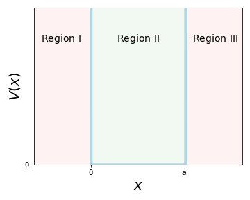
We will now solve a specific example of the time-independent Schrödinger equation: the infinite square well (ISW). In this scenario, the potential is given by \(V(x)=0\) for \(0\leqslant x\leqslant a\) and \(V(x)=\infty\) for \(x<0\), \(x>a\) (everywhere else).

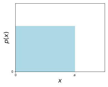
Classically, for \(E\neq0\), the particle bounces back and forth between the two walls and has equal probability to be everywhere in the well.

In quantum mechanics, we have to solve the TISE. Let's look at the various regions:

• Regions I & III: \(\psi_I(x)=\psi_{II}(x)=0\) as \(V=\infty\). This is straight forward.

• Region II: As \(V=0\), the TISE simplifies to

\[-\frac{\hbar^2}{2m}\frac{\mathrm{d}^2}{dx^2}\psi=E\psi\]

We can re-write this as \(\frac{\mathrm{d}^2}{dx^2}\psi=-k^2\psi\), where we have defined \(k\equiv\frac{\sqrt{2mE}}{\hbar}\) and assumed \(E>0\). This looks a lot like a classical harmonic oscillator (without damping or driving) \(F=m\cdot a=m\frac{\mathrm{d}^2x}{dt^2}=-kx\), which helps us to guess a solution: \(\psi(x)=A\sin kx+B\cos kx\) (the general solution of a harmonic oscillator (HO)). Now, how do we find the explicit form of \(\psi(x)\)? Are there any restricions we can find for \(A\), \(B\) and \(k\)? Let us try to use boundary conditions, as we usually do for differential equations! Because \(|\psi|^2=0\) for \(x<0\) and \(x>a\), we can use \(\psi(0)=\psi(a)=0\), such that \(\psi\) and \(\frac{\mathrm{d}\psi}{dx}\) are continuous¹. This leads us to the solutions for \(x=0\): \(\psi(0)=A\sin0+B\cos0=B\rightarrow B=0\) and \(\psi(x)=A\sin kx\) For \(x=a\): \(\psi(a)=A\sin ka\) and as \(A\neq0\), \(\sin ka=0\). Hence the possible solutions for \(ka=0,\pm\pi,\pm2\pi,\pm3\pi,\dots\), where we will neglect \(ka=0\), as it would give us the trivial solution \(\psi(x)=0\), which is unphysical, as it's not normalizable. The general solution therefore is \(k_n=\frac{n\pi}{a}\), with \(n\in\mathbb{Z}^*\). Let's look at the simplest example:

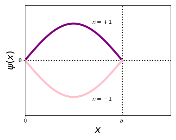
Clearly, both are the same solution, as a phase in QM makes (almost) no difference. Hence, the general solution simplifies to \(\psi_n(x)=A_n\sin\left(\frac{n\pi x}{a}\right)\), with \(k_n=\frac{n\pi}{a}\) and \(n\in\mathbb{N}^*\).

Now that we have the general solution for the ISW, let's find the normalization \(A_n\)²

\[\int_{-\infty}^{+\infty}|\psi_n|^2\mathrm{d}x=1=\int_{0}^{a}|A_n|^2\sin^2\left(\frac{n\pi x}{a}\right)\mathrm{d}x=\]

\[=\int_{0}^{a}|A_n|^2\frac{1}{2}\left(1-\cos\left(\frac{2n\pi x}{a}\right)\right)\mathrm{d}x=\]

\[=|A_n|^2\frac{1}{2}\left.\left[x-\frac{\sin\left(\frac{2n\pi x}{a}\right)}{\frac{2n\pi}{a}}\right]\right\vert_0^a=|A_n|^2\frac{a}{2}\]

If we choose the appropriate phase, we hence get \(A_n=\sqrt{\frac{2}{a}}\) and the general solution for the ISW is

\[\psi_n(x)=\sqrt{\frac{2}{a}}\sin\left(\frac{n\pi x}{a}\right)\]

Now, let us plug in the \(\psi_n\)'s into the TISE and find the energy³

\[-\frac{\hbar^2}{2m}\frac{\mathrm{d}^2}{\mathrm{d}x^2}\psi_n=E_n\psi_n\]

\[-\frac{\hbar^2}{2m}\frac{\mathrm{d}^2}{\mathrm{d}x^2}\sqrt{\frac{2}{a}}\sin\left(\frac{n\pi x}{a}\right)=\]

\[-\frac{\hbar^2}{2m}\sqrt{\frac{2}{a}}\left(\frac{n\pi x}{a}\right)^2(-1)\sin\left(\frac{n\pi x}{a}\right)=\frac{\hbar^2n^2\pi^2}{2ma^2}\sqrt{\frac{2}{a}}\sin\left(\frac{n\pi x}{a}\right)\]

Hence \(E_n=\frac{\hbar^2n^2\pi^2}{2ma^2}\). We of course knew that already, as we had initially defined \(E_n=\frac{k_n^2\hbar^2}{2m}\). We can now draw the first few solutions

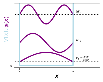
Remarkably, there is always energy, which we call the zero point energy. This is unlike anything we know from classical physics. Another general observation of these so-called bound states is that if we go up \(+1\) in energy, it adds \(+1\) in the number of nodes. Let's look at some more properties of the ISW:

1. Intuitively, the zero point energy is the kinetic energy from the curvature of the wavefunction. Higher energy states have more curvature and therefore more energy.

2. Higher energy states have more nodes.

3. The wavefunctions have symmetries about \(\frac{a}{2}\), even for \(n=1,3,5,\dots\) and odd for \(n=2,4,6,\dots\). This is very useful for finding solutions of integrals!

4. \(\psi_n\) are orthonormal \(\int\psi_n^*\psi_m\mathrm{d}x=\delta_{n,m}\).

5. \(\psi_n\) also form a complete set! How do we find the Fourier coefficients \(c_n\)? We use the properties of orthonormality and completeness:

   \[\int\psi_n^*(x)f(x)\mathrm{d}x=\int\psi_n^*(x)\sum_{m}c_m\psi_m(x)=\sum_{m}c_m\int\psi_n^*(x)\psi_m(x)\mathrm{d}x\]
   \[\Rightarrow c_n=\int\psi_n^*(x)f(x)\mathrm{d}x\]

Example:

Calculate \(\langle x\rangle\) for \(\psi_1(x)\) of the infinite square well. \(\langle x\rangle=\int\psi_1^*(x)\hat{x}\psi_1(x)\mathrm{d}x\). We can either continue by plugging in \(\psi_1(x)\) or by looking for symmetries. We note that \(\psi_1(x)\) has an even symmetry about \(x=\frac{a}{2}\), while \(x\) unfortunately does not have a symmetry around around the same point.

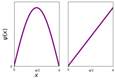
We can however use a trick and write \(x=(x-\frac{a}{2})+\frac{a}{2}\). Now, the part in the bracket is anti-symmetric around \(\frac{a}{2}\) and the second part is symmetric around \(\frac{a}{2}\)!

\[\langle x\rangle=\int\psi_1^*(x)\left(x-\frac{a}{2}\right)\psi_1(x)\mathrm{d}x+\int\psi_1^*(x)\frac{a}{2}\psi_1(x)\mathrm{d}x=\]

\[=\frac{a}{2}\int\psi_1^*(x)\psi_1(x)\mathrm{d}x=\frac{a}{2}\]

In the first line we have used the fact that the first integral is zero, as we have an even, an odd, and an even function in the integral, which overall gives the integral over an odd function. The result \(\langle x\rangle=\frac{a}{2}\) makes intuitive sense, as \(|\psi_1|^2\) is a \(\cos^2\) centered around \(\frac{a}{2}\). This clearly demonstrates that symmetries can greatly simplify our calculations!

Example:

Calculate \(\langle p\rangle\) for \(\psi_1(x)\) of the infinite square well.

\[\langle p\rangle=\int\psi_1^*(x)\hat{p}\psi_1(x)\mathrm{d}x = \int\psi_1^*(x)\frac{\hbar}{i}\frac{\mathrm{d}}{\mathrm{d}x}\psi_1(x)\mathrm{d}x=0\]

This is again the case because we have two even (\(\psi_1\)) and one odd (\(\frac{\mathrm{d}}{\mathrm{d}x}\)) functions.

Theorem

\(\langle p\rangle\) is zero for any localized, stationary state!

Suppose \(\langle p\rangle\neq0\), what would happen to \(\langle x\rangle\)? It would move as a function of time. However, we have seen that \(\langle x\rangle\) is independent of time for stationary states. Only superpositions of stationary states can have \(\langle p\rangle\neq0\).

Example:

Calculate \(\langle x\rangle\) for \(\Psi=\frac{1}{\sqrt{2}}\left(\psi_1+\psi_2\right)\). Let's first sketch the wavefunction:

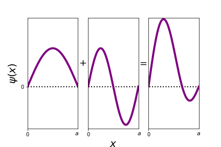
Now, let us check if there are any useful symmetries: \(\psi_1\) is even and \(\psi_2\) odd around \(\frac{a}{2}\), however \(\Psi\) is neither even nor odd. We therefore have to calculate \(\langle x\rangle\).

\[\langle x\rangle=\frac{1}{2}\int\left(\psi_1^*+\psi_2^*\right)x\left(\psi_1+\psi_2\right)\mathrm{d}x=\]

\[=\frac{1}{2}\int\psi_1^*x\psi_1\mathrm{d}x+\frac{1}{2}\int\psi_2^*x\psi_2\mathrm{d}x+\frac{1}{2}\int\psi_1x\psi_2\mathrm{d}x+\frac{1}{2}\int\psi_2x\psi_1\mathrm{d}x=\frac{a}{2}+\int\psi_1\psi_2x\mathrm{d}x\]

We next have to integrate by parts, which is an example in your homework.

Example:

Calculate \(\langle p^2\rangle\) for \(\psi_1\).

\[\langle p^2\rangle=\int\psi_1^*(x)\frac{\hbar^2}{-1}\frac{\mathrm{d}^2}{\mathrm{d}x^2}\psi_1(x)\mathrm{d}x=-\hbar^2\int\psi_1^*(x)\frac{-2m}{\hbar^2}E_1\psi_1(x)\mathrm{d}x=2mE_1\]

Example:

You are given a wavefunction \(\Psi(x,0)\), which is \(A\) for \(0<x<a\) and \(0\) otherwise. Find \(\Psi(x,t)\) for \(t>0\).

We first normalize \(\Psi(x,0)\) and obtain \(A=\frac{1}{\sqrt{a}}\). We then proceed to find \(c_n\)

\[c_n=\int_0^a\psi_n^*(x)\Psi(x,0)\mathrm{d}x=\frac{1}{\sqrt{a}}\sqrt{\frac{2}{a}}\int_0^a\sin\left(\frac{n\pi x}{a}\right)\mathrm{d}x=\]

\[=\frac{\sqrt{2}}{a}\frac{a}{n\pi}\left.\left[-\cos\left(\frac{n\pi x}{a}\right)\right]\right\vert_0^a=\frac{\sqrt{2}}{n\pi}\left(1-\cos(n\pi)\right)=\frac{2\sqrt{2}}{\pi}\frac{1}{n}\]

for \(n\) odd. The time-dependent wavefunction therefore is

\[\Psi(x,t)=\sum_{n,\mathrm{odd}}e^{-iE_nt/\hbar}\frac{4}{\pi\sqrt{a}n}\sin\left(\frac{n\pi x}{a}\right)\]

There is a problem however with \(\Psi(x,0)\) - it is discontinuous and hence leads to an infinitly large energy. Nevertheless, this is a useful example on how to add the time-dependence to a wavefunction.

---

1. Why do we want that? Think about the kinetic energy: \(\langle T\rangle=\int\psi^*\frac{-\hbar^2}{2m}\frac{\mathrm{d}^2}{\mathrm{d}x^2}\psi\mathrm{d}x\). If \(\psi\) was not continuous, this would imply \(\langle E\rangle\rightarrow\infty\). Note that for \(V=\infty\), \(\frac{\mathrm{d}\psi}{\mathrm{d}x}\) can be discontinuous and have \(\langle E\rangle\neq0\) (see example in the Book). ↩

2. We use the identities \(\sin^2x=\frac{1}{2}(1-\cos2x))\) and \(\int\cos x\,\mathrm{d}x=\sin x\). ↩

3. \(\frac{\mathrm{d}}{\mathrm{d}x}\sin x=\cos x\) and \(\frac{\mathrm{d}}{\mathrm{d}x}\cos x=-\sin x\) ↩