The Schrödinger equation

Week 1, Lecture 2

Let's look at some more details and properties of the wavefunction \(\Psi\):

• \(\Psi(x,t)\) is a complex valued function that obeys the TDSE.

• \(\int_a^b |\Psi(x,t)|^2 \,\mathrm{d}x\) is the probability of finding the particle between \(a\) and \(b\).

• \(\int_{-\infty}^{+\infty} |\Psi(x,t)|^2 \,\mathrm{d}x = ?\) \(\rightarrow\) It has to be equal to \(1\), as the particle has to be somewhere. This is called the normalization of the wavefunction.

Example:

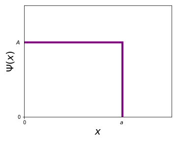
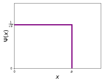
You're given the wavefunction of a particle with \(\Psi(x,0)=A\) for \(0<x<a\) and \(\Psi(x,0)=0\) otherwise. Now you need to calculate \(A\). It's always good to start with a sketch:

Now, in order to find \(A\), let's use the normalization:

\[\int_{-\infty}^{+\infty} |\Psi(x,0)|^2 \,\mathrm{d}x = \int_0^a |A|^2 \,\mathrm{d}x = a\cdot|A|^2 = 1\]

\[|A|^2=\frac{1}{a} \rightarrow A=\frac{1}{\sqrt{a}}\]

In the above example, is the answer we obtained the only valid answer? What about \(A=-\frac{1}{\sqrt{a}}\), \(A=\frac{i}{\sqrt{a}}\) or \(A=\frac{1}{i\sqrt{a}}\)? These are also correct answers for \(A\)! The most general answer is \(A=\frac{e^{i\theta}}{\sqrt{a}}\), where \(\theta\) can be any number. We conclude that \(\Psi\) is not unique, only up to an arbitrary phase factor!

Fortunately, this overall phase factor has no influence on the outcome of any measurements. For example, if we add a phase to our wavefunction \(\Psi\) and obtain a new wavefunction \(\Psi'\):

\[\Psi'=e^{i\theta}\Psi \rightarrow |\Psi'|^2=e^{-i\theta}\Psi^*e^{i\theta}\Psi=|\Psi|^2.\]

Example:

The wavefunction of particle is given as \(\Psi(x,0)=Ae^{-\lambda x^2}\). Find \(A\)!

\[\int_{-\infty}^{+\infty} |\Psi(x,0)|^2 \,\mathrm{d}x = |A|^2 \int_{-\infty}^{+\infty} e^{-2\lambda x^2} \,\mathrm{d}x =\]

In order to make our lives easier, we can substitute \(u=\sqrt{2\lambda}x\) and \(\mathrm{d}x=\frac{\mathrm{d}u}{\sqrt{2\lambda}}\).

\[= |A|^2 \int_{-\infty}^{+\infty} \frac{1}{\sqrt{2\lambda}} e^{-u^2}\,\mathrm{d}u = |A|^2 \frac{\sqrt{\pi}}{\sqrt{2\lambda}}\]

Here we've used the Gaussian integral \(\int_{-\infty}^{+\infty} e^{-x^2}\,\mathrm{d}x = \sqrt{\pi}\). Finally, we can use the normalization again \(|A|^2 \frac{\sqrt{\pi}}{\sqrt{2\lambda}} = 1\) and get as the general solution \(A = e^{i\theta} \left(\frac{2\lambda}{\pi}\right)^{1/4}\).

We've learned that \(\Psi(x,0)\) is normalized, so what about \(\Psi(x,t)\)? Do we need to recalculate the normalization for every \(t\)? The good news is we don't! The TDSE preserves the normalization (see below, as well as section 1.4 in the Book for the proof). What type of \(\Psi\)'s are good? Of course we need them to go to zero at infinity, as otherwise the integral of the normalization would diverge. For example, \(\Psi = e^x\) or \(\Psi = constant\) are not good solutions. We will require our wavefunctions to be \(\Psi=0\) for \(x\rightarrow\pm\infty\).

Evolution of the normalization in time

The normalization of the wavefunction is given by \(\int_{-\infty}^{+\infty} |\Psi(x,t)|^2 \,\mathrm{d}x = 1\). Let's see how it evolves over time:

\[\frac{\mathrm{d}}{\mathrm{d}t}\int_{-\infty}^{+\infty} |\Psi(x,t)|^2 \,\mathrm{d}x = \int_{-\infty}^{+\infty} \frac{\partial}{\partial t} |\Psi(x,t)|^2 \,\mathrm{d}x\]

We can use the product rule \(\frac{\partial}{\partial t}|\Psi|^2 = \frac{\partial}{\partial t}(\Psi^*\Psi)=\Psi^*\frac{\partial\Psi}{\partial t}+\frac{\partial\Psi^*}{\partial t}\Psi\)¹ and the TDSE, as well as the complex conjugate of the TDSE:

\[\frac{\partial\Psi}{\partial t}=\frac{i\hbar}{2m}\frac{\partial^2\Psi}{\partial x^2}-\frac{i}{\hbar}V\cdot\Psi\]

\[\frac{\partial\Psi^*}{\partial t}=-\frac{i\hbar}{2m}\frac{\partial^2\Psi^*}{\partial x^2}+\frac{i}{\hbar}V\cdot\Psi^*\]

to obtain

\[\frac{\partial}{\partial t} |\Psi|^2 = \Psi^*\left(\frac{i\hbar}{2m}\frac{\partial^2\Psi}{\partial x^2}-\frac{i}{\hbar}V\Psi\right)\cdot\left(-\frac{i\hbar}{2m}\frac{\partial^2\Psi^*}{\partial x^2}+\frac{i}{\hbar}V\Psi^*\right)\Psi=\]

\[=\frac{i\hbar}{2m}\left(\Psi^*\frac{\partial^2\Psi}{\partial x^2}-\frac{\partial^2\Psi^*}{\partial x^2}\Psi\right)=\frac{\partial}{\partial x}\left(\frac{i\hbar}{2m}\left(\Psi^*\frac{\partial\Psi}{\partial x}-\frac{\partial\Psi^*}{\partial x}\Psi\right)\right)\]

\[\Rightarrow\frac{\mathrm{d}}{\mathrm{d}t}\int_{-\infty}^{+\infty} |\Psi(x,t)|^2 \,\mathrm{d}x = \frac{i\hbar}{2m}\left.\left(\Psi^*\frac{\partial\Psi}{\partial x}-\frac{\partial\Psi^*}{\partial x}\Psi\right)\right|_{-\infty}^{+\infty} = 0\]

as for \(x\rightarrow\pm\infty\) we require \(\Psi\) to be zero. Hence we've demonstrated that the normalization is constant in time.

Expectation values

We have learned that \(\Psi(x,t)\) cannot predict the value of \(x\) in a single measurement. In statistics, the expectation value is the "average" value given by \(\langle x\rangle=\sum_i p(x_i)x_i\)

In quantum mechanics, the wavefunction \(\Psi\) can predict the expectation value deterministically:

\[\langle x(t)\rangle=\int_{-\infty}^{+\infty} x|\Psi(x,t)|^2\mathrm{d}x\]

Since \(x\) is a continuos variable here, the sum is substituted by an integral.

Example:

Same \(\Psi(x,0)\) from first example. Let's calculate \(\langle x\rangle\):

\[\langle x\rangle=\int_{-\infty}^{+\infty} x\frac{1}{a} \mathrm{d}x=\frac{1}{a}\int_{0}^{a}x\mathrm{d}x=\frac{1}{a} \left[\frac{x^2}{2}\right]_0^a=\frac{a}{2}\]

This is what we expected from looking at the sketch!

Example:

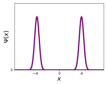
• What is \(\langle x\rangle\)? \(\rightarrow \langle x\rangle=0\)

• What are the most likely outcomes of a measurement? \(\rightarrow x=\pm a\)

• What is the probability to measure \(x=0\)? \(\rightarrow p(x=0)=0\)

\(\Rightarrow\) This is the same as in statistics: the most likely outcome is not always the average outcome!

We can of course also calculate other expectation values: for example \(\langle x^2(t)\rangle=\int_{-\infty}^{+\infty} x^2|\Psi(x,t)|^2\mathrm{d}x\). What about other interesting quantities, such as the velocity? As \(\Psi(x,0)\) contains all information about the state of a particle at time \(t=0\), we should be able to also get the expectation values for velocity. How do we use \(\Psi(x,0)\) to calculate \(\langle v(t=0)\rangle\)? What about \(\frac{\mathrm{d}\langle x\rangle}{\mathrm{d}t}\)?

\[\frac{\mathrm{d}\langle x\rangle}{\mathrm{d}t} = \int_{-\infty}^{+\infty} x\frac{\partial}{\partial t}|\Psi(x,t)|^2 \mathrm{d}x=\int_{-\infty}^{+\infty} x\left(\Psi^*\frac{\partial\Psi}{\partial t}+\frac{\partial\Psi^*}{\partial t}\Psi\right)\mathrm{d}x\]

By using the TDSE and some tricks (see Book) we finally obtain

\[\frac{\mathrm{d}\langle x\rangle}{\mathrm{d}t} = \frac{-i\hbar}{m}\int_{-\infty}^{+\infty} \Psi^*\frac{\partial}{\partial x}\Psi\mathrm{d}x\]

In quantum mechanics we usually don't work with the velocity, but rather with the momentum of a particle \(p=m\cdot v\)

\[\langle p\rangle = \frac{m\mathrm{d}\langle x\rangle}{\mathrm{d}t} = -i\hbar\int_{-\infty}^{+\infty} \Psi^*\frac{\partial}{\partial x}\Psi\mathrm{d}x\]

The information about the position is contained in \(|\Psi|^2\), while the information about the momentum is contained in the slope of \(\Psi\)!

Let's rewrite \(\langle x\rangle\) and \(\langle p\rangle\) in a suggestive form:

\[\langle x\rangle = \int_{-\infty}^{+\infty} \Psi^* x \Psi \mathrm{d}x\]

\[\langle p\rangle = \int_{-\infty}^{+\infty} \Psi^* \frac{\hbar}{i}\frac{\mathrm{d}}{\mathrm{d}x} \Psi \mathrm{d}x\]

Both of them have the form of a "sandwich" between \(\Psi^*\) and \(\Psi\) in the integral:

• to obtain \(\langle x\rangle\) you "sandwich" "\(x\)"
• to obtain \(\langle p\rangle\) you "sandwich" "\(\frac{\hbar}{i}\frac{\mathrm{d}}{\mathrm{d}x}\)"

We call \(x\) and \(\frac{\hbar}{i}\frac{\mathrm{d}}{\mathrm{d}x}\) operators that represent \(x\) and \(p\)! We can in fact express all properties (such as kinetic energy, potential energy, angular momentum, etc.) of a particle in terms of \(x\) and \(p\)!! The recipe for calculating the expectation value of any of these quantities \(Q(x,p)\) is to find the operator version of the quantity \(Q(x,p)\rightarrow Q\left(x,\frac{\hbar}{i}\frac{\mathrm{d}}{\mathrm{d}x}\right)\) and to put it in the sandwich:

\[\langle Q(x,p)\rangle = \int_{-\infty}^{+\infty} \Psi^* Q\left(x,\frac{\hbar}{i}\frac{\mathrm{d}}{\mathrm{d}x}\right) \Psi \mathrm{d}x\]

Example:

What is the expectation value for the kinetic energy \(T=\frac{p^2}{2m}\)

\[p^2\Rightarrow\frac{\hbar}{i}\frac{\partial}{\partial x}\frac{\hbar}{i}\frac{\partial}{\partial x}=\hbar^2\frac{\partial^2}{\partial x^2}\]

\[\langle T\rangle=\frac{\langle p^2\rangle}{2m}= -\frac{\hbar^2}{2m}\int_{-\infty}^{+\infty} \Psi^* \frac{\partial^2}{\partial x^2} \Psi \mathrm{d}x\]

Note that \(p\) is related to the slope of \(\Psi\), while \(T\) is related to the curvature of \(\Psi\)!

Let's take a step back: somehow \(\Psi(x,0)\) is not a function of time, but still contains information about the momentum of a particle!

Example:

Given \(\Psi_1(x,0)=Ae^{-\lambda x^2}\) and \(\Psi_2(x,0)=Ae^{ikx}e^{-\lambda x^2}\). Note that \(e^{ikx}\) is phase factor that is not constant! We immediately see that

\[|\Psi_1(x,0)|^2=|A|^2e^{-2\lambda x^2}=|\Psi_2(x,0)|^2\]

Let's first calculate \(\langle x\rangle\):

• For \(\Psi_1\): \(\langle x\rangle=|A|^2\int_{-\infty}^{+\infty}e^{-2\lambda x^2}x\mathrm{d}x=0\). This is easy to see as \(e^{-2\lambda x^2}\) is even around \(x=0\), while \(x\) is odd around \(x=0\). Because even\(\cdot\)odd\(=\)odd the integral is zero!²

• For \(\Psi_2\): \(\langle x\rangle=\int_{-\infty}^{+\infty}A^*e^{-ikx}e^{-\lambda x^2}xAe^{ikx}e^{-\lambda x^2}\mathrm{d}x=0\)

This is of course what we expected as we have the same \(|\Psi|^2\) for both wavefunctions. Now let's calculate \(\langle p\rangle\) next:

• For \(\Psi_1\): \(\langle p\rangle=\int_{-\infty}^{+\infty}A^*e^{-\lambda x^2}\frac{\hbar}{i}\frac{\mathrm{d}}{\mathrm{d}x}Ae^{-\lambda x^2}\mathrm{d}x=\)

\[=|A|^2\frac{\hbar}{i}\int_{-\infty}^{+\infty}e^{-\lambda x^2}(-2\lambda x)e^{-\lambda x^2}\mathrm{d}x=|A|^2\frac{\hbar}{i}(-2\lambda)\int_{-\infty}^{+\infty}xe^{-2\lambda x^2}\mathrm{d}x=0\]

• For \(\Psi_2\): \(\langle p\rangle=\int_{-\infty}^{+\infty}A^*e^{-ikx}e^{-\lambda x^2}\frac{\hbar}{i}\frac{\mathrm{d}}{\mathrm{d}x}Ae^{ikx}e^{-\lambda x^2}\mathrm{d}x\)

\[\frac{\mathrm{d}}{\mathrm{d}x}\left(e^{ikx}e^{-\lambda x^2}\right)=\frac{\mathrm{d}}{\mathrm{d}x}\left(e^{ikx-\lambda x^2}\right)=(ik-2\lambda x)e^{ikx-\lambda x^2}\]

Here the first term is new compared to \(\Psi_1\), while the second term is similar and \(\rightarrow 0\). We hence get

\[\langle p\rangle=|A|^2\int_{-\infty}^{+\infty}e^{-ikx}e^{-\lambda x^2}\frac{\hbar}{i}ike^{ikx}e^{-\lambda x^2}\mathrm{d}x=\hbar k\int_{-\infty}^{+\infty}|A|^2e^{-2\lambda x^2}\mathrm{d}x=\hbar k\int_{-\infty}^{+\infty}|\Psi_2|^2\mathrm{d}x=\hbar k\]

Interestingly, \(\Psi_2\) has a non-zero momentum, while \(\Psi_1\) does not. Where is the momentum hidden?

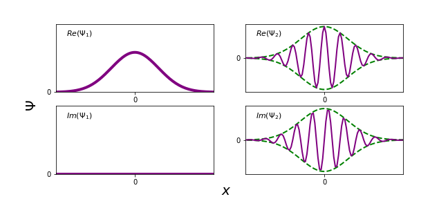
The spacing between peaks in oscillations in \(\Psi_2\) is \(\Delta x=\frac{2\pi}{k}=\lambda\). This might remind you of the de Broglie formula \(p=\frac{2\pi\hbar}{\lambda}\) but now we have \(\langle p\rangle=\hbar k=\frac{2\pi\hbar}{\lambda}\), with \(k=\frac{2\pi}{\lambda}\).

This calculations tells us that the second particle with wavefuction \(\Psi_2\) has a momentum given by the wavevector \(k\) in the exponential part (\(e^{ikx}\))!

Heisenberg uncertainty principle

You may have previously heard about the Heisenberg uncertainty principle:

\[\Delta x\cdot\Delta p\geqslant\hbar/2\]

What are these \(\Delta x\) and \(\Delta p\) in quantum mechanics? \(\Delta x\) is the standard deviation \(\sigma_x\) of an ensemble of measurements on particles all prepared in the state \(\Psi\).

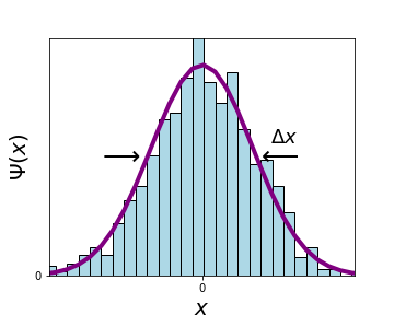
Given a wavefunction \(\Psi_1\) we can calculate the standard deviation as (see Book)

\[\sigma_x=\sqrt{\langle x^2\rangle-\langle x\rangle^2}\]

\[\sigma_p=\sqrt{\langle p^2\rangle-\langle p\rangle^2}\]

The Heisenberg uncertainty principle is

\[\sigma_x\cdot\sigma_p\geqslant\hbar/2\]

(we will use \(\Delta x\) and \(\sigma_x\) interchangeably). The uncertainty principle does not tell us the maximum accuracy with which we can measure the position of a particle, but rather how \(\sigma_x\) is related to \(\sigma_p\) for a given \(\Psi\)!

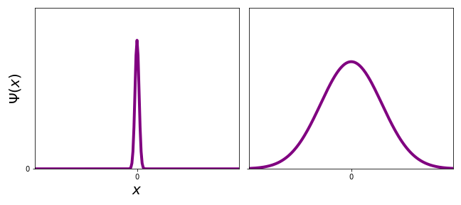
The momentum \(p\) is related to the wavelength of \(\Psi(x)\), or more accurately, how high a wavelength we need to construct \(\Psi(x)\) in a Fourier series. A sharp peak (left) contains many different \(k\)'s, hence leading to a larger \(\sigma_p\), while a broad peak (right) has a smaller \(\sigma_p\), as less \(k\)'s are needed to construct the peak.

---

1. \((f\cdot g)'=f'\cdot g+f\cdot g'\) and \(\frac{\mathrm{d}}{\mathrm{d}x}(u\cdot v)=\frac{\mathrm{d}u}{\mathrm{d}x}\cdot v+u\cdot\frac{\mathrm{d}v}{\mathrm{d}x}\) ↩

2. An odd function is defined as \(f(-x)=-f(x)\), while an even function is \(f(x)=f(-x)\). ↩