Week 3, lecture 7

The free particle

You might have noticed that we haven't discussed so far the simplest quantum system, which corresponds to the case where the potential vanishes everywhere, \(V(x)=0\) \(\forall x\). This system is known as the free particle.

As we will see in this lecture, this system is not as trivial as it might seem at first glance (in stark contract with the classical free particle, which is the first system you solve when learning about Newtonian's mechanics).

Its main problem is that the solutions of its Schrodinger equation turn out not to be normalisable, and hence cannot represent physical states. But we will be able to combine these solutions into a wave packet that can after all represent physical states.

The Schroedinger equation for the free particle

The time-independent Schroedinger equation for the free particle reads

\[-\frac{\hbar^2}{2m}\frac{d^2\psi(x)}{dx^2}=E\psi(x),~~{\rm Eq.}~[1]\]

which can also be expressed as

\[\frac{d^2\psi(x)}{dx^2}=-\frac{2mE}{\hbar^2}\psi(x),~~{\rm Eq.}~[2]\]

which is a second-order differential equation that we have to solve.

Info

For homogeneous second order differential equations, the general solution is the linear combination of two particular independent solutions. To find a particular solution, we could try a possible ansatz and see if it works. This general solution will depend on two integration constants, which need to be determined either by imposing the boundary conditions or the normalisation of the wave function.

You can then convince yourselves that the most general solution of Eq. [2] is given by:

\[\psi(x)=Ae^{ikx}+Be^{-ikx},~~{\rm where}~~k\equiv\sqrt{\frac{2mE}{\hbar^2}}\, , ~~{\rm Eq.}~[3]\]

where \(A\) and \(B\) are integration constants. To show this, note that \(e^{ikx}\) and \(e^{-ikx}\) are independent particular solutions of this differential equation, and hence the general solution will be its linear superposition.

For a given value of \(k\), the corresponding energies will be given by $$ E_k = \frac{\hbar^2 k^2}{2m} \, . $$ You can also determine the dispersion relations for these solutions, defined as the relation between the angular velocity \(\omega\) and \(k\): $$ E = h \nu = h \frac{\omega}{2\pi} = \hbar \omega = \frac{\hbar^2 k^2}{2m} $$ where we have used Planck's relation between energy and frequency, and hence the dispersion relation for these solutions will be given by $$ \omega = \frac{\hbar k^2}{2m} \, . $$

Information

The phase velocity of a wave is defined as \(v_{\rm phase}=\omega/k\). For these free-particle solutions, the phase velocity is $$ v_{\rm phase} = \frac{\omega}{k} = \frac{\hbar k}{2m} \, . $$
This phase velocity can be compared with the classical velocity associated by a particle with energy \(E=\hbar^2k^2/2m\): $$ v_{\rm classical} = \sqrt{\frac{2E}{m}} = \sqrt{\frac{2}{m}\frac{\hbar^2 k^2}{2m} }=\frac{\hbar k}{m} = v_{\rm phase}/2 \, . $$ This factor two of difference will be explained by the fact that free-particle solutions with fixed energy, as we will show, do not represent physical states. Once we define physical states by means of a wave packet, we will be able to connect the wave velocity with the classical result.

Note that the general solution of the free-particle Schroedinger equation, Eq. [3], can also be expressed as a linear combination of trigonometric functions. By recalling the relation between complex exponentials and trigonometric functions $$ \cos(x) = \frac{e^{ix}+e^{-ix}}{2} \, , \quad \sin(x) = \frac{e^{ix}-e^{-ix}}{2i} \, , $$ you can check that Eq. [2] can also be expressed as $$ \psi(x)=C\cos(kx)+D\sin(kx),~~{\rm where}~~k\equiv\sqrt{\frac{2mE}{\hbar^2}} \, $$ where \(C\) and \(D\) are other integration constants.

In contrast with the infinite well case, for the free particle system we don't have boundary conditions on the wavefunction, and therefore the energy \(E\) can take any positive value: the only contribution to the total energy is the kinetic energy, which is positive-definite. So in the case of the free particle system the energy is not quantised and can take a continuum of values.

As you can verify, in the limit \(x\rightarrow \pm\infty\) the wavefunction \(\psi(x)\) in Eq. [3] does not vanish but rather oscillates around zero. This feature has an important implication: the wavefunction corresponding to the free particle with fixed energy \(E\) cannot be normalized and therefore cannot represent a physical quantum state!

Recall

One of the fundamental axioms of quantum mechanics is that the wavefunction of physical states admits a probabilistic interpretation. Therefore, a wave function that cannot be normalized cannot be associated to a physical quantum state. Else we would find inconsistent situations, such as probabilities of specific outcomes of measurements being greater than 1.

The problem we are facing here is originated by assuming that the free particle will have associated a single value of the energy (as is the case for all solutions of the Schroedinger equation). This assumption leads to a wave function which is maximally delocalized: the particle has an equal probability to be found anywhere in space, including at infinity!

Actually, this is something that we could have expected if we had considered the Heisenberg uncertainty principle for position and momentum, which imposes the requirement that $$ \Delta x \Delta p \ge \frac{\hbar}{2} \, , $$ where \(\Delta x\) and \(\Delta p\) represent our uncertainty in the knowledge in the position and linear momentum of our particle.

In the case of the free particle, if we have solutions with well-defined energy \(E\) then we know perfectly well the value of the kinetic energy \(T=E\) and hence of its linear momentum. This implies that \(\Delta p = 0\), and hence \(\Delta x \ge (\hbar/ 2\Delta p) \to \infty\): we don't have any information about the position of the particle!

For all we know, a free particle with well-defined energy could be found anywhere in the whole Universe. We say that this quantum state is maximally delocalised, and such states cannot be normalised since the particle has a finite probability to be found at \(|x|\to \infty\).

You can verify explicitely that these solutions of the free-particle Schroedinger equation are not normalisable. Considering for example one of the particular solutions and attempt to evaluate its normalization constant: $$ \psi(x)=Ae^{ikx},~~{\rm where}~~k=\sqrt{\frac{2mE}{\hbar^2}} $$ so we attempt to integrate the square of the wave function over the available range of values of \(x\): $$ \int_{-\infty}^{+\infty}\psi^*(x)\psi(x)dx=\int_{-\infty}^{+\infty}Ae^{-ikx}Ae^{ikx}dx=\int_{-\infty}^{+\infty}A^2dx \to \infty $$

Therefore, there does not exist any finite value of \(A\) for which the free-particle wave function with fixed energy can be normalised.

Does this mean that we cannot find physical wavefunctions for the free-particle system? Certainly not, since a non-interacting particle is a well-defined physical system and one should be able to find acceptable wavefunctions in quantum mechanics as we do in classical physics.

The way to find physical wavefunctions is to combine solutions with different energies. In such case, \(\Delta p\) will take a finite value and hence \(\Delta x\) can be finite as well, by virtue of the Heisenberg principle.

And if a particle is localised (as is the case for any finite \(\Delta x\)), one will be able to construct normalisable wave functions.

The wave packet

To solve this problem, we are going to use the property that the eigenvectors \(\psi_k(x)\) of the Schrodinger equation of a free particle form a complete basis (more about this in future lectures, when we present the formalism of quantum theory).

Therefore, we can combine these eigenvectors \(\psi_k(x)\) linearly in some clever manner in order to construct a physically valid (and hence normalisable) wavefunction. Specifically, we need to construct a wave function \(\psi(x)\) for the free particle that vanishes at \(|x|\to \infty\) and hence can be normalised.

The superposition principle of quantum mechanics tells me that if the eigenvectors of the free particle Schroedinger equation are given by

\[\psi_k(x)=Ae^{ikx},~~{\rm where}~~k=\pm \sqrt{\frac{2mE}{\hbar^2}}\]

then the most general wave function for this quantum system \(\Psi(x)\) will be given by the following linear superposition:

\[\Psi(x)=\sum_k c_k \psi_k(x),~~{\rm Eq.~[4]}\]

for any complex values of the coefficients \(c_k\) and where the sum runs over all possible values of the wave vector \(k\).

Recall that this property, the superposition principle, is fully general and applies to any quantum system, not only the free particle. As we will see when we discuss the formalism of quantum mechanics, the reason is that quantum states are elements of a vector space and hence can be linearly combined and the result is guaranteed to yield another valid quantum state.

Info

The wave function \(\Psi(x)\) constructed in Eq. [4] is not a solution of the Schroedinger equation, despite being defined as a linear superposition of the Hamiltonian eigenfunctions \(\psi_k(x)\). That is, you can check explicitely that \(\hat{H}\Psi(x)\ne E \Psi(x)\) for any value of the energy \(E\). This implies that \(\Psi(x)\) does not have a well-defined value of its energy and hence should be possible to normalise it, following the considerations above about the Heisenberg uncertainty principle.

In the case of a quantum system like the free particle, where its solutions are not quantized (as shown by the fact that the wave number \(k\) can take any value), one should replace a sum by an integral (which after all is nothing but an infinite sum over continuous elements).

Taking this feature into account, we can construct the most general wavefunction for a free particle as follows:

\[\Psi(x)=\frac{1}{\sqrt{2\pi}}\int_{-\infty}^{+\infty} \,dk\,\phi(k)e^{ikx},~~{\rm Eq.}~[5]\]

In this expression, \(\phi(k)\) is a general function of the wave number \(k\) that corresponds to the continuum analog of the coefficients \(c_k\) in the discrete case. The factor \(1\sqrt{2\pi}\) as we will see has been factored out of \(\phi(k)\) for convenience.

Eq. [5] is known as a wave packet, since it is a linear combination of individual waves with well-defined frequency (that is, with fixed energy and wavelength). Note that the wave packet itself does not have a unique energy of wavelenght. Difference choices of \(\phi(k)\) will then result into different shapes of the wave packet.

What we need to do now is to determine for which functions \(\phi(k)\) the wave function of our system, Eq. [5], will be normalizable and thus will admit the probabilistic inerpretation which is required for physical quantum systems.

Warning

Note that even if the original wave functions \(\psi_k(x)\) were not integrable, it is possible to combine them linearly such that their superposition is indeed integrable, if one chooses the wave number profile \(\phi(k)\) in a clever manner.

A powerful strategy to determine the function \(\phi(k)\) is to exploit the orthogonality property for the solutions of the Schroedinger equation for the free particle, which tells us that:

\[\int_{-\infty}^{+\infty}dx\,e^{ikx}e^{-ik'x}=2\pi\delta(k-k'),~~{\rm Eq.}~[6]\]

in terms of the Dirac delta function.

Information

The Dirac delta function (technically, it is a distribution rather than a function) is zero if \(k\ne k'\) and infinite for \(k=k'\), and its action is defined by the following condition $$ \int_{-\infty}^{+\infty}dk\, f(k)\,\delta(k-k')=f(k') $$ for any general function \(f(k)\). The Dirac delta function is the analog for the continuous case of the Kroneker delta \(\delta_{mn}\) that we have been using so far.

Eq. [6] is the analog, in the case of continuous (non quantized) spectra, of the usual orthogonality relations between the solutions of the Schroedinger equation that you have already encountered in systems where the energy levels are quantised, such as the infinite well and the quantum harmonic oscillator, where we used:

\[\int_{-\infty}^{+\infty}\psi_{l}^{*}(x)\psi_{n}(x)dx=\delta_{ln}\]

where \(l\) and \(n\) were the quantum numbers labeling each independent solution of the Schrodinguer equation.

We can use this orthogonality property to determine the function \(\phi(k)\). To see this, start from Eq. [5], multiply by \(e^{-ik'x}\), and integrate over all allowed values of \(x\):

\[ \int_{-\infty}^{+\infty}dx\,e^{-ik'x} \Psi(x)=\int_{-\infty}^{+\infty}dx\,e^{-ik'x}\left( \frac{1}{\sqrt{2\pi}}\int_{-\infty}^{+\infty} \,dk\,\phi(k)e^{ikx}\right)\]

and then we can simplify the right hand side of the equation above by using the defining property of the Dirac delta function

\[ \int_{-\infty}^{+\infty}dx\,e^{-ik'x} \frac{1}{\sqrt{2\pi}}\int_{-\infty}^{+\infty} \,dk\,\phi(k)e^{ikx} = \frac{1}{\sqrt{2\pi}} \int_{-\infty}^{+\infty} dk\, \phi(k)\int_{-\infty}^{+\infty}dx\,e^{-i(k'-k)}\, \]

\[ \frac{1}{\sqrt{2\pi}} \int_{-\infty}^{+\infty} dk\, \phi(k) \left( 2\pi \delta(k-k') \right) = \sqrt{2\pi} \phi(k') \]

By using this property, we therefore find that the function \(\phi(k)\) is given by

\[\phi(k)=\frac{1}{\sqrt{2\pi}}\int_{-\infty}^{+\infty}\Psi(x)e^{-ikx}dx,~~{\rm Eq.}~[7]\]

in other words, \(\phi(k)\) is the Fourier transform of the original wave function \(\Psi(x)\).

This result implies that given a choice for the desired shape of the wave function of my free-particle system, \(\Psi(x)\), by using Eq. [7] I can always determine the shape of the required function \(\phi(k)\) in wave vector space required to construct a wave pack from a linear combination of the solutions of the Schroedinger equation.

We will now show an explicit example of this, the so-called Gaussian wave packet where the function \(\phi(k)\) is chosen to ensure a Gaussian wave function in position space.

The Gaussian wave packet:

Consider free particle with the following wave function at \(t=0\)

\[\Psi(x,0)=Ae^{-ax^2}\]

where \(A\) and \(a\) are real and positive constants. We would like to find the function \(\phi(k)\) that defines the wave packet leading to \(\Psi(x,0)\) and determine how the properties of the resulting wave packet vary with time.

(a) First of all, we want to normalize \(\Psi(x,0)\), that is, find the value of the constant \(A\):

\[\int_{-\infty}^{+\infty} dx\, |\Psi(x,0)|^2=|A|^2\int_{-\infty}^{+\infty}e^{-2ax^2}dx=1\]

\[|A|^2\sqrt{\frac{\pi}{2a}}=1~~\rightarrow~~|A|=\left(\frac{2a}{\pi}\right)^{1/4}\]

Note that here I will take \(A\) to be real, but we could have always multiplied it by an arbitrary complex phase.

(b) Next we want to evaluate the function \(\phi(k)\) that ensures the desired Gaussian profile of the wave packet: $$ \phi(k)=\frac{A}{\sqrt{2\pi}}\int_{-\infty}^{+\infty}e^{-ax^2}e^{-ikx}dx $$

\[ \phi(k)=\frac{1}{(2\pi a)^{1/4}}e^{-k^2/4a} \]

where we have used the following result for definite Gaussian integrals

\[ \int_{-\infty}^{+\infty}e^{-(ax^2+bx)}dx=\sqrt{\frac{\pi}{a}}e^{b^2/4a} \]

(c) Now that we have found \(\phi(k)\) and the normalisation constant \(A\), we can determine the time evolution of the wave packet:

\[\Psi(x,t)=\frac{1}{\sqrt{2\pi}}\frac{1}{(2\pi a)^{1/4}}\int_{-\infty}^{+\infty}e^{-k^2/4a}e^{i(kx-(\frac{\hbar k^2}{2m})t)}dk=\frac{1}{\sqrt{2\pi}}\frac{1}{(2\pi a)^{1/4}}\int_{-\infty}^{+\infty}e^{-[(\frac{1}{4a}+i\frac{\hbar t}{2m})k^2-ixk]}dk\]

\[\Psi(x,t)=\left(\frac{2a}{\pi}\right)^{1/4}\frac{e^{-ax^2/(1+2i\hbar at/m)}}{\sqrt{1+2i\hbar at/m}}\]

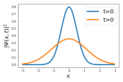
You can then evaluate the corresponding probability distribution \(|\Psi(x,t)|^2\): you can verify that one ends up with a Gaussian distribution ceentered at \(x=0\) and with variance increasing with time (see below).

In other words, while \(x=0\) remains at all times the most likely position of the particle, as time goes on, the probability of finding the particle far from the origin increases rapidly. So the wave packet spreads out as time goes on.

This discussion illustrates how a wave packet can be constructed from a superposition of sinusoidal functions (each with different frequency) with their ampitude modulated by the function \(\phi(k)\). While the individual waves are not normalised, their combination via a wave packet is normalisable and thus can represent a physical state.

Group and phase velocity

An interesting question in this context is what is the velocity of the particle whose wave function is represented by the wave packet. We saw before that the phase velocity of a wave function with fixed \(E=\hbar^2k^2/2m\) was $$ v_{\rm phase} = \frac{\omega}{k} = \frac{\hbar k}{2m} $$ but now in a wave packet we combine waves with different values of \(k\), what will be the resulting velocity?

A wave packet consists on individual ripples contained within an envelope. What corresponds to the particle velocity in this case is not the speed of the individual ripples, which is called the phase velocity but rather the speed of the envelope itself, which is known as the group velocity of the wave packet.

For the wave function of a free particle in quantum mechanics, the group velocity is twice the phase velocity, and matches the classical particle speed. We will now demonstrate this important property.

Let us consider the general wave function of the free particle system given by a wave packet with envelope \(\phi(k)\):

\[ \Psi(x,t)=\frac{1}{\sqrt{2\pi}}\int_{-\infty}^{+\infty} \,dk\,\phi(k)e^{i(kx-\omega t)} \]

where the wave angular velocity \(\omega=\hbar k^2/2m\) is different for each of the modes \(k\) that constitute the wave packet.

We will assume that \(\phi(k)\) is peaked around some \(k_0\), else different components of the wave packet travel at very different velocities and the whole notion of group velocity becomes meaningless.

We can then taylor-expand the frequency around \(k=k_0\), since far from it the envelope function \(\phi(k)\) is very small and thus the integrand will vanish. We then have

\[ \omega(k)\simeq \omega_0 + \omega'_0(k-k_0) \, ,\quad \omega'_0\equiv \frac{d\omega(k)}{dk}\Bigg|_{k=k_0} \, . \]

Now we can change variables to \(s=k-k_0\), so that the integration range is centered around the maximum of \(\phi(k)\). After doing some algebra, we find that the time-dependent wave function \(\Psi(x,t)\) describing our particle can be expressed as

\[ \Psi(x,t)\simeq \frac{1}{\sqrt{2\pi}}e^{i(k_0x - \omega_0t)} \int_{-\infty}^{\infty} ds\,\phi(k_0+s)e^{is(x-\omega'_0t)} \]

We see that our wave function is composed by a sinusoidal wave (the ripples) travelling at speed \(\omega_0/k_0\) which is modulated by the integral, an envelope which is a function of \(x-\omega'_0t\), hence propagating at speed \(\omega'_0\).

We thus see that the phase velocity of this wave packet is

\[ v_{\rm phase}=\frac{\omega}{k}\Bigg|_{k=k_0} = \frac{\hbar k_0}{2m} \]

while the group velocity of the wave packet is

\[ v_{\rm group} = \frac{d\omega}{dk}\Bigg|_{k=k_0}=\frac{\hbar k_0}{m} \]

For our free particle, the dispersion relation between angular frequency and wave number is \(\omega=\hbar k^2/2m\) and hence we find that the group velocity is equal to the classical velocity of the wave, which in turn is twice the phase velocity: $$ v_{\rm classical} = v_{\rm group} = 2v_{\rm phase} $$ which is a reassuring result: the group velocity of a free particle constructed as a narrowly peaked wave packet coincides with the classical expectation for the particle's velocity.

The fact that a narrowly peaked wave packet can be visualised as a dominant sinusoidal wave (the ripples) modulated by an envelope can be better visualised in the graphic below. We show a gaussian wave packet, where a Gaussian envelope \(\phi(k)\propto e^{-bk^2}\) leads to a Gaussian wave function in position space:

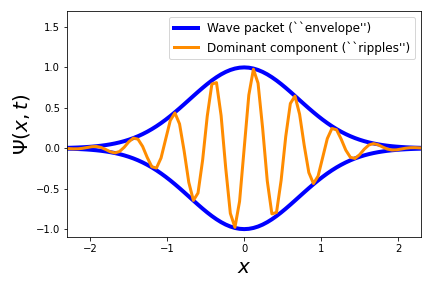
The dominant sinusoidal component (the ripples) travels with velocity \(v_{\rm phase}=\hbar k_0/2m\), while the envelope travels at twice that velocity, $v_{\rm group} = \hbar k_0/m $, which corresponds to the classical velocity that a particle with kinetic energy \(E=\hbar^2k^2/2m\) would have.

To summarise, it is thus now clear how by choosing \(\phi(k)\) we can ensure that our free-particle quantum states are normalisable and this physical: we need to select an initial condition for the wave function that is normalisable, as was the case in the previous exercise with \(\psi(x,0)=Ae^{-ax^2}\).