The Schrödinger equation¶

Week 1, Lecture 1

Let's start with the time-dependent Schrödinger equation (TDSE), named after the Austrian physicist Erwin Schrödinger (1887-1961, Nobel prize in physics 1933):

\[-\frac{\hbar^2}{2m}\frac{\partial^2\Psi(x,t)}{\partial x^2} + V(x,t)\cdot\Psi(x,t)=i\hbar\frac{\partial\Psi(x,t)}{\partial t}\]

where \(\Psi\) is called the wavefunction, \(m\) is the mass, \(V\) the potential a particle is in and the constant \(\hbar=h/2\pi=1.054572\times10^{-34}\) is called the reduced Planck constant. Max Planck was a German physicist (1858-1947, Nobel prize 1918). In quantum mechanics (QM), \(\Psi\) describes all properties of a particle. If you're given the wavefunction of a system at \(t=0\), \(\Psi(x,0)\), and \(V\), then the TDSE tells you how to calculate \(\Psi(x,t)\) for all times \(t\).

Recall

This is of course similar to Newton's second law: in classical mechanics, given \(x(0)\), \(v(0)\) and \(V\), you can calculate \(x(t)\) for all times \(t\) in the future.

What are the properties of \(\Psi(x)\)? Is it real or complex valued? What does it mean and how do we use it? This is essentially the content of the rest of the course: you will learn to interpret \(\Psi\) and use it to make predictions and determine characteristics of a quantum system.

Statistical interpretation (or Born rule)¶

This is named after a German physicist, Max Born (1882-1970), who won the Nobel prize in physics in 1954 for the statistical interpretation of quantum mechanics. Using the wavefunction, we can calculate the probability of finding a particle between \(x\) and \(x+\mathrm{d}x\) at a time \(t\) according to

\[|\Psi(x,t)|^2\mathrm{d}x\]

Let's draw this as a graph to better understand

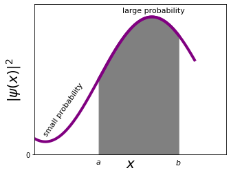
and we can then calculate the probability of finding (measuring) the particle between \(a\) and \(b\) at a given time \(t\) just like defined above

\[\int_a^b |\Psi(x,t)|^2 \,\mathrm{d}x\]

It is important to note here, that from the statistical interpretation of QM we can conclude that while the Schrödinger equation tells us with absolute certainty how \(\Psi(x,t)\) will evolve given \(\Psi(x,0)\), the wavefunction \(\Psi(x,t)\) itself only gives us probabilistic information about the outcome of a measurement. This is a fundamental feauture of QM: even if you have all possible information about a particle (i.e. you know \(\Psi(x,t)\)), quantum theory cannot (in principle!) predict the outcome of a measurement. It will only give you probabilistic, not deterministic, information on a measurement. This is in stark contrast to classical mechanics! If you are given \(x(0)\), v(0) and V(x,t), you can precisely predict the outcome of every measurement you could ever perform.

Even for a particle that is standing still, it is not possible to precisely predict the outcome of a measurement in QM!

So how can we use \(\Psi\) then?

Example:

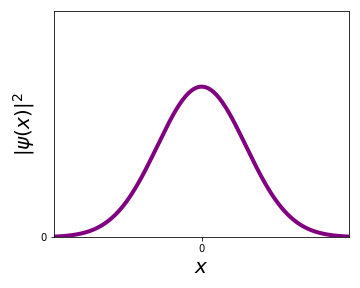
Let's perform an experiment: I'll give you \(N\) particles that I have all prepared in the same wavefunction \(\Psi(x)\). One by one, you measure the position of each particle, which every time gives you a (different) probablistic result. This allows you to build up a histogram:

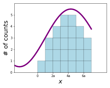
With enough measurements, after you've gathered a large set of measurements, the histogram will converge to a probability distribution given by \(|\Psi(x)|^2\).

Quantum measurement¶

So far we've learned about the wavefunction and how it allows us to predict the probability of a measurement outcome. But what happens to \(\Psi(x,t)\) after a measurement? The Schrödinger equation does not tell us what happens to \(\Psi(x,t)\) during a measurement! All we know (so far) is to interpret \(|\Psi|^2\) as the probability of a measurement outcome. So how do we know what \(\Psi\) is after a measurement? Since the SE does not tell us, let's perform an experiment and see what happens.

Example:

In this example I will give you a bag filled with particles, all in the same state \(\Psi\). Now, take one out and measure it. After that, immediately measure the same particle again and again. What happens is the following:

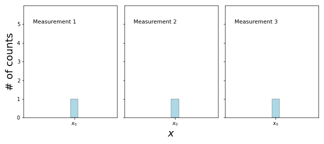
You can see that if you measure the same particle over and over again, you will always get the same answer! Remember, the situation is very different if you measure a particle from the bag, take another one and measure it and so on, even though they are all prepared in the same state \(\Psi\):

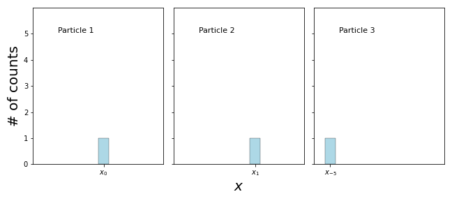
After we do enough measurements and we add everything up, we will eventually arrive at the distribution given by the wavefunction

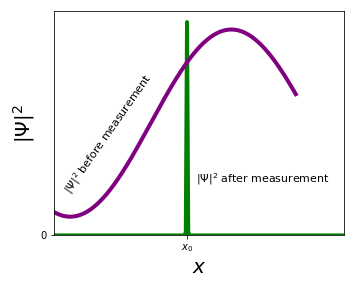
What does this experiment tell us about the \(\Psi(x)\) after the measurement? The only way that a measurement will always give you the same result is if \(\Psi(x)\) is sharply peaked around \(x_0\), where the first measurement found the particle! We say that the measurement has collapsed the wavefunction.

Recap: for you to find out what \(\Psi\) is (or at least \(|\Psi|^2\)), you need to perform measurements on a large ensemble of identically prepared particles. If you have just one particle, you cannot find \(\Psi\). This is a fundamental difference between classical and quantum mechanics.

Classical mechanics: A particle's state is described completely by its position and velocity. With one particle you can know everything about its state by measuring \(x\) and \(v\).
Quantum mechanics: A particle's state is described by its wavefunction \(\Psi\). If you only have one particle, you cannot find \(\Psi\), as each measurement only gives you partial information on \(\Psi\) and "destroys" \(\Psi\) after you measure it.

This is not only strange, but also really useful. For example, the "no cloning theorem" (Book, Chapter 12) allows you to use this to transmit secret information using quantum states in an asbolute secure way. This is often also called quantum cryptography.

Summary¶

\(\Psi(x,t)\) contains all information about the state of a particle.
Given \(\Psi(x,0)\) and \(V(x,t)\), the TDSE tells you \(\Psi(x,t)\) for all times \(t>0\), as long as you don't measure.
If you measure, the outcome is not deterministic, but probabilistic! Each measurement can give a different answer on where the particle is, with a statistical probability of \(\int_a^b |\Psi(x,t)|^2 \,\mathrm{d}x\) for finding the particle between \(a\) and \(b\).
After a measurement that gives you an outcome \(x_0\), the wavefunction collapses to a sharp peak centered around \(x_0\).

One can say that there are two quantum worlds: the deterministic Schrödinger equation and the probabilistic measurement.

Finally, let's discuss where the particle was before the measurement. There are competing ideas around this and the two most important views are:

Orthodox position: The particle wasn't anywhere. The measurement projected the particle into a position. In other words, the measurement creates the result. This is often referred to as the Copenhagen interpretation.
Realist position: The particle was already at position \(x_0\) prior and independently of the measurement - we just couldn't know. From a classical point of view this makes sense and Einstein famously said about this: "God does not play dice". There is one major issue with this position, namely that this would mean that QM is an incomplete theory. Therefore, there must exist another ("better") theory that includes a set of hidden variables (not accessible in QM), which completely describes every measurement outcome deterministically.

In fact, there exists a theorem, called Bell's theorem (after John Bell, 1928-1990), that allows one to experimentally test if there is any theory that could include these hidden variables and therefore be a complete theory (see Chapter 12 in the Book). Many experiments have tested this theorem, particularly in the 1970's¹ and 1980's² and also recently in Delft³^,⁴, and all show that no such (local) hidden variable theory can exist.

S. J. Freedman and J. F. Clauser, Phys. Rev. Lett. 28, 938 (1972) ↩
A. Aspect, P. Grangier, and G. Roger, Phys. Rev. Lett. 47, 460 (1981) ↩
B. Hensen, et al., Nature 526, 682 (2015) ↩
I. Marinković, A. Wallucks, R. Riedinger, S. Hong, M. Aspelmeyer, and S. Gröblacher, Phys. Rev. Lett. 121, 220404 (2018) ↩